The R Formula Method: The Bad Parts

No Recycling

As a corollary to the point above, there is no way to recycle the terms between models that share the same formula and data/environment. For example, if I fit a CART model to a data set with many predictors, the random forest model (theoretically) shouldn’t need to recreate the same terms information about the design matrix. If the model function has the non-formula interface (e.g., mod_func(x, y)), this can make it easier. However, many do not.

Also, suppose that one of the pre-processing steps is computationally expensive. We’d like to be able to store the state of the results and then add another layer of computations (perhaps as a separate object).

Formulas and Wide Datasets

The terms object saves a matrix with as many rows as formula variables and at least as many columns (depending on interactions, etc). Most of this data is zero and a non–sparse representation is used. The current framework was built in a time where there was more focus on interactions, nesting and other operations on a small scale.

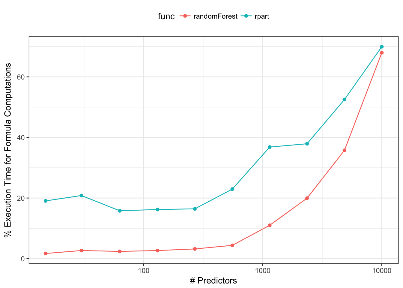
It is unlikely that models would have hundreds of interaction terms, but now it is not uncommon to have hundreds or thousands of main effects. As the number of predictors increases, this takes up an inordinate amount of execution time. For simple randomForest or rpart calls, the formula/terms work can account for most of the execution time. For example, we can calculate how much time functions spend generating the model matrix relative to the total execution time. For rpart and randomForest, we used the default arguments and did the calculations with a simulated data set of 200 data points and varying numbers of predictors:

This is especially problematic for ensemble models. For example, ipred:::ipredbagg creates an ensemble of rpart trees. Since rpart only has a formula method, the footprint of the bagged model object can become very large if X trees are contained in the ensemble. Alternatively, randomForest.formula takes the approach of generating the terms once and feeding the model frame to randomForest.default. This does not work for rpart since there is no non-formula method exposed. Some functions (e.g., lm, survival::coxph) have arguments that can be used to prevent the terms and similar objects from being returned. This saves space but prevents new samples from being predicted. A little more detail can be found here.

One issue is the "factors" attribute of the terms object (discussed in the previous post). This is a non-sparse matrix that has a row for each predictor in the formula and a column for each model term (e.g. main effects, interactions, etc.). The purpose of this object is to know which predictors are involved in which terms.

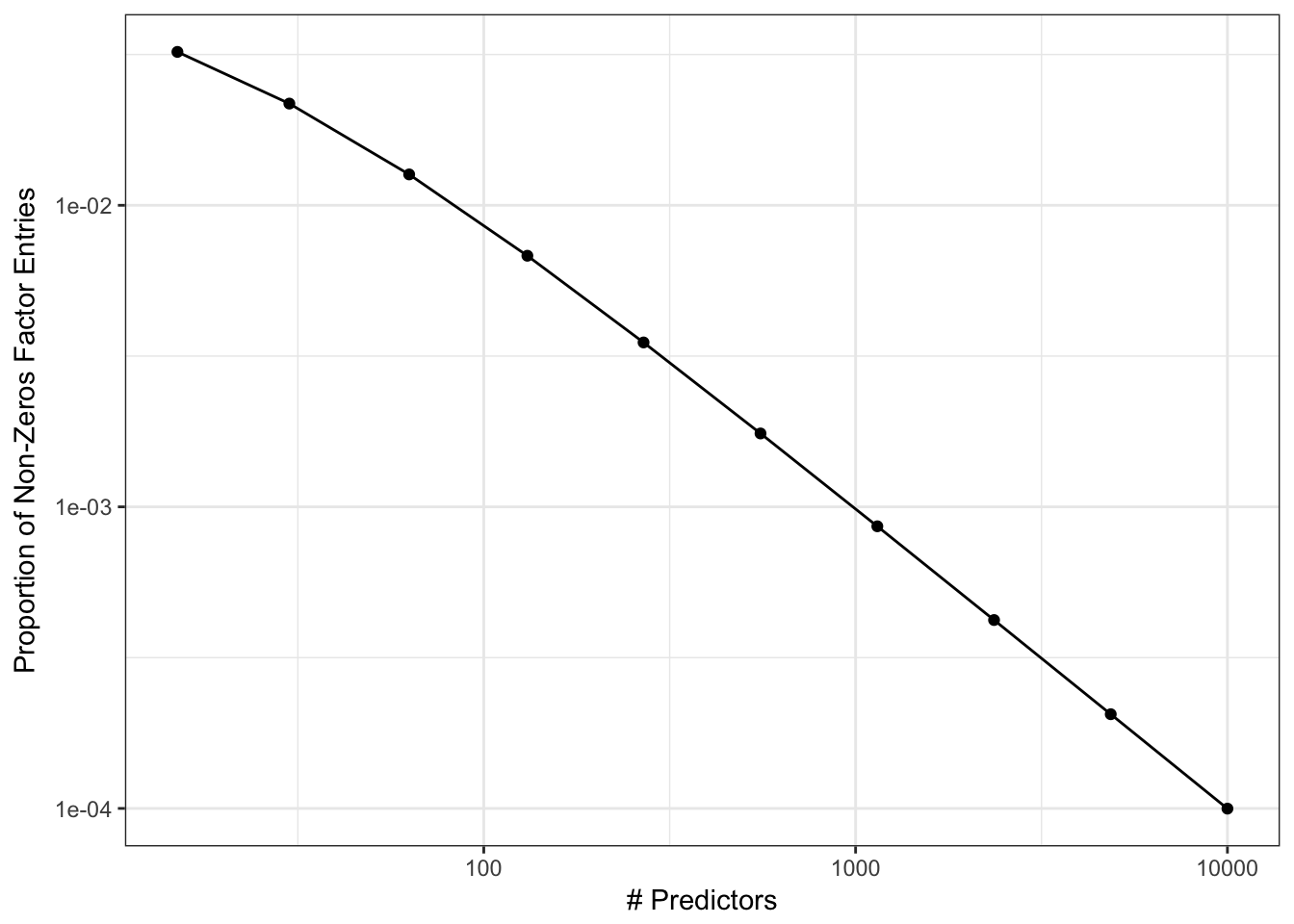
The issue is that this matrix can get very large and usually has a high proportion of zeros. For example:

mod3 <- lm(Sepal.Width ~ Petal.Width + Petal.Length*Species, data = iris)
fact_mat <- attr(mod3$terms, "factors")
fact_mat

##              Petal.Width Petal.Length Species Petal.Length:Species
## Sepal.Width            0            0       0                    0
## Petal.Width            1            0       0                    0
## Petal.Length           0            1       0                    1
## Species                0            0       1                    1

As the number of predictors increases, the rate of ones is likely to approach a value close to zero very quickly. For example:

Again, it is doubtful that a model with a large number of predictors will have a correspondingly large number of high-level interactions (see the Pareto principle applied to modeling).

Variable Roles

Some packages have implemented extensions of the basic formula. There are cases when formula are needed for specific sub-models. For example, a random coefficient model can be fit with the lmer function. In this case, a model is specified for a particular clustering variable (e.g., a subject in a clinical trial). The code is an example of how lmer syntax works:

# ?lme4::lmer
lmer(Reaction ~ Days + (Days | Subject), data = sleepstudy)

Here Subject is important to the model-fitting routine, but not as a predictor. Similarly, the Bradley-Terry model can be used to model competitions and contests. A model on a set of boxers in a series of contests can include terms for their reach:

BTm(outcome = 1, player1 = winner, player2 = loser, 
    formula = ~reach[..] + (1 | ..), 
    data = boxers)

Another extension of basic formulas comes from the modeltools and mboost packages. The function mboost::mob fits a tree-based model with regression models in the terminal nodes. For this model, a separate list of predictors are used as splitting variables (to define the tree structure) and another set of regression variables that are modeled in the terminal nodes. An example of this call is:

# mboost::mob (using the modeltools package for formulas)
mob(diabetes ~ glucose | pregnant + mass +  age,
    data = PimaIndiansDiabetes)

The commonality between these three examples is that there are variables that are critical to the model but do not play the role of standard regression terms. For lmer, Subject is the independent experimental unit. For mob, we have variables to be used for splitting, etc.

There are similar issues on the left-hand side of the formula. When there are multivariate outcomes, different packages have different approaches:

# ?aggregate the mean of two variables by month
aggregate(cbind(Ozone, Temp) ~ Month, data = airquality, mean)

# grouped binomial data:
glm(cbind(events, nonevents) ~ x, family = binomial)

# pls::plsr, 
pls(sensory ~ chemical, data = oliveoil)
# sensory and chemical are 2D arrays in the oliveoil data frame

The overall point here is that, for the most part, the formula method assumes that there is one variable on the left-hand side of the tilde and that the variables on the right-hand side are predictors (exceptions are discussed below). One can envision other roles that columns could play in the analysis of data. Besides the examples given above, variables could be used for

• outcomes
• predictors
• stratification
• data for assessing model performance (e.g., loan amount to compute expected loss)
• conditioning or faceting variables (e.g., lattice or ggplot2)
• random effects or hierarchical model ID variables
• case weights
• offsets
• error terms (limited to Error in the aov function)

The last three items on this list are currently handled in formulas as “specials” or have existing functions. For example, when the model function has a weights argument, the current formula/terms frame work uses a function (model.weights) to extract the weights, and also makes sure that the weights are not included as covariates. The same is true for offsets.