With roots dating back to at least 1662 when John Graunt, a London merchant, published an extensive set of inferences based on mortality records, survival analysis is one of the oldest subfields of Statistics [1]. Basic life-table methods, including techniques for dealing with censored data, were discovered before 1700 [2], and in the early eighteenth century, the old masters - de Moivre working on annuities, and Daniel Bernoulli studying competing risks for the analysis of smallpox inoculation - developed the modern foundations of the field [2]. Today, survival analysis models are important in Engineering, Insurance, Marketing, Medicine, and many more application areas. So, it is not surprising that R should be rich in survival analysis functions. CRAN’s Survival Analysis Task View, a curated list of the best relevant R survival analysis packages and functions, is indeed formidable. We all owe a great deal of gratitude to Arthur Allignol and Aurielien Latouche, the task view maintainers.
Looking at the Task View on a small screen, however, is a bit like standing too close to a brick wall - left-right, up-down, bricks all around. It is a fantastic edifice that gives some idea of the significant contributions R developers have made both to the theory and practice of Survival Analysis. As well-organized as it is, however, I imagine that even survival analysis experts need some time to find their way around this task view. Newcomers - people either new to R or new to survival analysis or both - must find it overwhelming. So, it is with newcomers in mind that I offer the following narrow trajectory through the task view that relies on just a few packages: survival, ggplot2, ggfortify, and ranger
The survival package is the cornerstone of the entire R survival analysis edifice. Not only is the package itself rich in features, but the object created by the Surv() function, which contains failure time and censoring information, is the basic survival analysis data structure in R. Dr. Terry Therneau, the package author, began working on the survival package in 1986. The first public release, in late 1989, used the Statlib service hosted by Carnegie Mellon University. Thereafter, the package was incorporated directly into Splus, and subsequently into R.
ggfortify enables producing handsome, one-line survival plots with ggplot2::autoplot.
ranger might be the surprise in my very short list of survival packages. The ranger() function is well-known for being a fast implementation of the Random Forests algorithm for building ensembles of classification and regression trees. But ranger() also works with survival data. Benchmarks indicate that ranger() is suitable for building time-to-event models with the large, high-dimensional data sets important to internet marketing applications. Since ranger() uses standard Surv() survival objects, it’s an ideal tool for getting acquainted with survival analysis in this machine-learning age.
Load the data
This first block of code loads the required packages, along with the veteran dataset from the survival package that contains data from a two-treatment, randomized trial for lung cancer.
library(survival)
library(ranger)
library(ggplot2)
library(dplyr)
library(ggfortify)

#------------
data(veteran)
head(veteran)
## trt celltype time status karno diagtime age prior
## 1 1 squamous 72 1 60 7 69 0
## 2 1 squamous 411 1 70 5 64 10
## 3 1 squamous 228 1 60 3 38 0
## 4 1 squamous 126 1 60 9 63 10
## 5 1 squamous 118 1 70 11 65 10
## 6 1 squamous 10 1 20 5 49 0The variables in veteran are: * trt: 1=standard 2=test * celltype: 1=squamous, 2=small cell, 3=adeno, 4=large * time: survival time in days * status: censoring status * karno: Karnofsky performance score (100=good) * diagtime: months from diagnosis to randomization * age: in years * prior: prior therapy 0=no, 10=yes
Kaplan Meier Analysis
The first thing to do is to use Surv() to build the standard survival object. The variable time records survival time; status indicates whether the patient’s death was observed (status = 1) or that survival time was censored (status = 0). Note that a “+” after the time in the print out of km indicates censoring.
# Kaplan Meier Survival Curve
km <- with(veteran, Surv(time, status))
head(km,80)
## [1] 72 411 228 126 118 10 82 110 314 100+ 42 8 144 25+
## [15] 11 30 384 4 54 13 123+ 97+ 153 59 117 16 151 22
## [29] 56 21 18 139 20 31 52 287 18 51 122 27 54 7
## [43] 63 392 10 8 92 35 117 132 12 162 3 95 177 162
## [57] 216 553 278 12 260 200 156 182+ 143 105 103 250 100 999
## [71] 112 87+ 231+ 242 991 111 1 587 389 33To begin our analysis, we use the formula Surv(futime, status) ~ 1 and the survfit() function to produce the Kaplan-Meier estimates of the probability of survival over time. The times parameter of the summary() function gives some control over which times to print. Here, it is set to print the estimates for 1, 30, 60 and 90 days, and then every 90 days thereafter. This is the simplest possible model. It only takes three lines of R code to fit it, and produce numerical and graphical summaries.
km_fit <- survfit(Surv(time, status) ~ 1, data=veteran)
summary(km_fit, times = c(1,30,60,90*(1:10)))
## Call: survfit(formula = Surv(time, status) ~ 1, data = veteran)
##
## time n.risk n.event survival std.err lower 95% CI upper 95% CI
## 1 137 2 0.985 0.0102 0.96552 1.0000
## 30 97 39 0.700 0.0392 0.62774 0.7816
## 60 73 22 0.538 0.0427 0.46070 0.6288
## 90 62 10 0.464 0.0428 0.38731 0.5560
## 180 27 30 0.222 0.0369 0.16066 0.3079
## 270 16 9 0.144 0.0319 0.09338 0.2223
## 360 10 6 0.090 0.0265 0.05061 0.1602
## 450 5 5 0.045 0.0194 0.01931 0.1049
## 540 4 1 0.036 0.0175 0.01389 0.0934
## 630 2 2 0.018 0.0126 0.00459 0.0707
## 720 2 0 0.018 0.0126 0.00459 0.0707
## 810 2 0 0.018 0.0126 0.00459 0.0707
## 900 2 0 0.018 0.0126 0.00459 0.0707#plot(km_fit, xlab="Days", main = 'Kaplan Meyer Plot') #base graphics is always ready
autoplot(km_fit)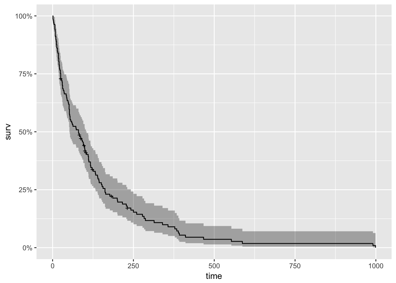
Next, we look at survival curves by treatment.
km_trt_fit <- survfit(Surv(time, status) ~ trt, data=veteran)
autoplot(km_trt_fit)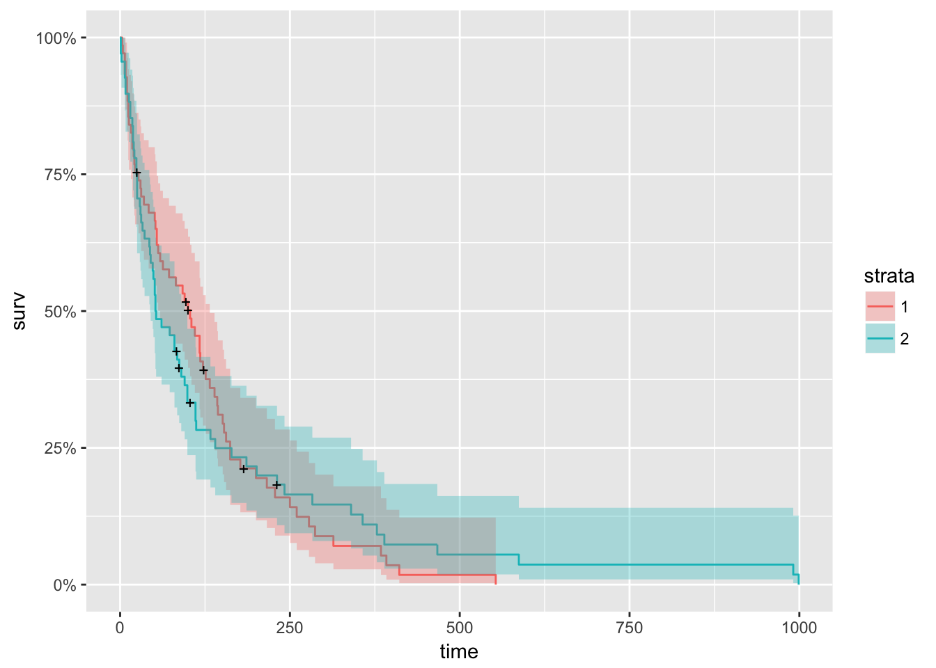
And, to show one more small exploratory plot, I’ll do just a little data munging to look at survival by age. First, I create a new data frame with a categorical variable AG that has values LT60 and GT60, which respectively describe veterans younger and older than sixty. While I am at it, I make trt and prior into factor variables. But note, survfit() and npsurv() worked just fine without this refinement.
vet <- mutate(veteran, AG = ifelse((age < 60), "LT60", "OV60"),
              AG = factor(AG),
              trt = factor(trt,labels=c("standard","test")),
              prior = factor(prior,labels=c("N0","Yes")))

km_AG_fit <- survfit(Surv(time, status) ~ AG, data=vet)
autoplot(km_AG_fit)
Although the two curves appear to overlap in the first fifty days, younger patients clearly have a better chance of surviving more than a year.
Cox Proportional Hazards Model
Next, I’ll fit a Cox Proportional Hazards Model that makes use of all of the covariates in the data set.
# Fit Cox Model
cox <- coxph(Surv(time, status) ~ trt + celltype + karno                   + diagtime + age + prior , data = vet)
summary(cox)
## Call:
## coxph(formula = Surv(time, status) ~ trt + celltype + karno +
## diagtime + age + prior, data = vet)
##
## n= 137, number of events= 128
##
## coef exp(coef) se(coef) z Pr(>|z|)
## trttest 2.946e-01 1.343e+00 2.075e-01 1.419 0.15577
## celltypesmallcell 8.616e-01 2.367e+00 2.753e-01 3.130 0.00175 **
## celltypeadeno 1.196e+00 3.307e+00 3.009e-01 3.975 7.05e-05 ***
## celltypelarge 4.013e-01 1.494e+00 2.827e-01 1.420 0.15574
## karno -3.282e-02 9.677e-01 5.508e-03 -5.958 2.55e-09 ***
## diagtime 8.132e-05 1.000e+00 9.136e-03 0.009 0.99290
## age -8.706e-03 9.913e-01 9.300e-03 -0.936 0.34920
## priorYes 7.159e-02 1.074e+00 2.323e-01 0.308 0.75794
## ---
## Signif. codes: 0 '***' 0.001 '**' 0.01 '*' 0.05 '.' 0.1 ' ' 1
##
## exp(coef) exp(-coef) lower .95 upper .95
## trttest 1.3426 0.7448 0.8939 2.0166
## celltypesmallcell 2.3669 0.4225 1.3799 4.0597
## celltypeadeno 3.3071 0.3024 1.8336 5.9647
## celltypelarge 1.4938 0.6695 0.8583 2.5996
## karno 0.9677 1.0334 0.9573 0.9782
## diagtime 1.0001 0.9999 0.9823 1.0182
## age 0.9913 1.0087 0.9734 1.0096
## priorYes 1.0742 0.9309 0.6813 1.6937
##
## Concordance= 0.736 (se = 0.03 )
## Rsquare= 0.364 (max possible= 0.999 )
## Likelihood ratio test= 62.1 on 8 df, p=2e-10
## Wald test = 62.37 on 8 df, p=2e-10
## Score (logrank) test = 66.74 on 8 df, p=2e-11cox_fit <- survfit(cox)
#plot(cox_fit, main = "cph model", xlab="Days")
autoplot(cox_fit)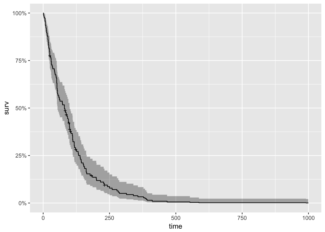
Note that the model flags small cell type, adeno cell type and karno as significant. However, some caution needs to be exercised in interpreting these results. While the Cox Proportional Hazard’s model is thought to be “robust”, a careful analysis would check the assumptions underlying the model. For example, the Cox model assumes that the covariates do not vary with time. In a vignette [12] that accompanies the survival package Therneau, Crowson and Atkinson demonstrate that the Karnofsky score (karno) is, in fact, time-dependent so the assumptions for the Cox model are not met. The vignette authors go on to present a strategy for dealing with time dependent covariates.
Data scientists who are accustomed to computing ROC curves to assess model performance should be interested in the Concordance statistic. The documentation for the survConcordance() function in the survival package defines concordance as “the probability of agreement for any two randomly chosen observations, where in this case agreement means that the observation with the shorter survival time of the two also has the larger risk score. The predictor (or risk score) will often be the result of a Cox model or other regression” and notes that: “For continuous covariates concordance is equivalent to Kendall’s tau, and for logistic regression is is equivalent to the area under the ROC curve.”
To demonstrate using the survival package, along with ggplot2 and ggfortify, I’ll fit Aalen’s additive regression model for censored data to the veteran data. The documentation states: “The Aalen model assumes that the cumulative hazard H(t) for a subject can be expressed as a(t) + X B(t), where a(t) is a time-dependent intercept term, X is the vector of covariates for the subject (possibly time-dependent), and B(t) is a time-dependent matrix of coefficients.”
The plots show how the effects of the covariates change over time. Notice the steep slope and then abrupt change in slope of karno.
aa_fit <-aareg(Surv(time, status) ~ trt + celltype +
                 karno + diagtime + age + prior ,
                 data = vet)
aa_fit
## Call:
## aareg(formula = Surv(time, status) ~ trt + celltype + karno +
## diagtime + age + prior, data = vet)
##
## n= 137
## 75 out of 97 unique event times used
##
## slope coef se(coef) z p
## Intercept 0.083400 3.81e-02 1.09e-02 3.490 4.79e-04
## trttest 0.006730 2.49e-03 2.58e-03 0.967 3.34e-01
## celltypesmallcell 0.015000 7.30e-03 3.38e-03 2.160 3.09e-02
## celltypeadeno 0.018400 1.03e-02 4.20e-03 2.450 1.42e-02
## celltypelarge -0.001090 -6.21e-04 2.71e-03 -0.229 8.19e-01
## karno -0.001180 -4.37e-04 8.77e-05 -4.980 6.28e-07
## diagtime -0.000243 -4.92e-05 1.64e-04 -0.300 7.65e-01
## age -0.000246 -6.27e-05 1.28e-04 -0.491 6.23e-01
## priorYes 0.003300 1.54e-03 2.86e-03 0.539 5.90e-01
##
## Chisq=41.62 on 8 df, p=1.6e-06; test weights=aalen#summary(aa_fit) # provides a more complete summary of results
autoplot(aa_fit)
Random Forests Model
As a final example of what some might perceive as a data-science-like way to do time-to-event modeling, I’ll use the ranger() function to fit a Random Forests Ensemble model to the data. Note however, that there is nothing new about building tree models of survival data. Terry Therneau also wrote the rpart package, R’s basic tree-modeling package, along with Brian Ripley. See section 8.4 for the rpart vignette [14] that contains a survival analysis example.
ranger() builds a model for each observation in the data set. The next block of code builds the model using the same variables used in the Cox model above, and plots twenty random curves, along with a curve that represents the global average for all of the patients. Note that I am using plain old base R graphics here.
# ranger model
r_fit <- ranger(Surv(time, status) ~ trt + celltype +
                     karno + diagtime + age + prior,
                     data = vet,
                     mtry = 4,
                     importance = "permutation",
                     splitrule = "extratrees",
                     verbose = TRUE)

# Average the survival models
death_times <- r_fit$unique.death.times
surv_prob <- data.frame(r_fit$survival)
avg_prob <- sapply(surv_prob,mean)

# Plot the survival models for each patient
plot(r_fit$unique.death.times,r_fit$survival[1,],
     type = "l",
     ylim = c(0,1),
     col = "red",
     xlab = "Days",
     ylab = "survival",
     main = "Patient Survival Curves")

#
cols <- colors()
for (n in sample(c(2:dim(vet)[1]), 20)){
  lines(r_fit$unique.death.times, r_fit$survival[n,], type = "l", col = cols[n])
}
lines(death_times, avg_prob, lwd = 2)
legend(500, 0.7, legend = c('Average = black'))
The next block of code illustrates how ranger() ranks variable importance.
vi <- data.frame(sort(round(r_fit$variable.importance, 4), decreasing = TRUE))
names(vi) <- "importance"
head(vi)
## importance
## karno 0.0903
## celltype 0.0323
## diagtime -0.0012
## trt -0.0013
## prior -0.0027
## age -0.0037Notice that ranger() flags karno and celltype as the two most important; the same variables with the smallest p-values in the Cox model. Also note that the importance results just give variable names and not level names. This is because ranger and other tree models do not usually create dummy variables.
But ranger() does compute Harrell’s c-index (See [8] p. 370 for the definition), which is similar to the Concordance statistic described above. This is a generalization of the ROC curve, which reduces to the Wilcoxon-Mann-Whitney statistic for binary variables, which in turn, is equivalent to computing the area under the ROC curve.
cat("Prediction Error = 1 - Harrell's c-index = ", r_fit$prediction.error)## Prediction Error = 1 - Harrell's c-index = 0.3087233An ROC value of .68 would normally be pretty good for a first try. But note that the ranger model doesn’t do anything to address the time varying coefficients. This apparently is a challenge. In a 2011 paper [16], Hamad observes:
However, in the context of survival trees, a further difficulty arises when time–varying effects are included. Hence, we feel that the interpretation of covariate effects with tree ensembles in general is still mainly unsolved and should attract future research.
I believe that the major use for tree-based models for survival data will be to deal with very large data sets.
Finally, to provide an “eyeball comparison” of the three survival curves, I’ll plot them on the same graph.The following code pulls out the survival data from the three model objects and puts them into a data frame for ggplot().
# Set up for ggplot
kmi <- rep("KM",length(km_fit$time))
km_df <- data.frame(km_fit$time,km_fit$surv,kmi)
names(km_df) <- c("Time","Surv","Model")

coxi <- rep("Cox",length(cox_fit$time))
cox_df <- data.frame(cox_fit$time,cox_fit$surv,coxi)
names(cox_df) <- c("Time","Surv","Model")

rfi <- rep("RF",length(r_fit$unique.death.times))
rf_df <- data.frame(r_fit$unique.death.times,avg_prob,rfi)
names(rf_df) <- c("Time","Surv","Model")

plot_df <- rbind(km_df,cox_df,rf_df)

p <- ggplot(plot_df, aes(x = Time, y = Surv, color = Model))
p + geom_line()
For this data set, I would put my money on a carefully constructed Cox model that takes into account the time varying coefficients. I suspect that there are neither enough observations nor enough explanatory variables for the ranger() model to do better.
This four-package excursion only hints at the Survival Analysis tools that are available in R, but it does illustrate some of the richness of the R platform, which has been under continuous development and improvement for nearly twenty years. The ranger package, which suggests the survival package, and ggfortify, which depends on ggplot2 and also suggests the survival package, illustrate how open-source code allows developers to build on the work of their predecessors. The documentation that accompanies the survival package, the numerous online resources, and the statistics such as concordance and Harrell’s c-index packed into the objects produced by fitting the models gives some idea of the statistical depth that underlies almost everything R.
Some Tutorials and Papers
For a very nice, basic tutorial on survival analysis, have a look at the Survival Analysis in R [5] and the OIsurv package produced by the folks at OpenIntro.
Look here for an exposition of the Cox Proportional Hazard’s Model, and here [11] for an introduction to Aalen’s Additive Regression Model.
For an elementary treatment of evaluating the proportional hazards assumption that uses the veterans data set, see the text by Kleinbaum and Klein [13].
For an exposition of the sort of predictive survival analysis modeling that can be done with ranger, be sure to have a look at Manuel Amunategui’s post and video.
See the 1995 paper [15] by Intrator and Kooperberg for an early review of using classification and regression trees to study survival data.
References
For convenience, I have collected the references used throughout the post here.
[1] Hacking, Ian. (2006) The Emergence of Probability: A Philosophical Study of Early Ideas about Probability Induction and Statistical Inference. Cambridge University Press, 2nd ed., p. 11
[2] Andersen, P.K., Keiding, N. (1998) Survival analysis Encyclopedia of Biostatistics 6. Wiley, pp. 4452-4461 [3] Kaplan, E.L. & Meier, P. (1958). Non-parametric estimation from incomplete observations, J American Stats Assn. 53, pp. 457–481, 562–563. [4] Cox, D.R. (1972). Regression models and life-tables (with discussion), Journal of the Royal Statistical Society (B) 34, pp. 187–220.
[5] Diez, David. Survival Analysis in R, OpenIntro
[6] Klein, John P and Moeschberger, Melvin L. Survival Analysis Techniques for Censored and Truncated Data, Springer. (1997)
[7] Wright, Marvin & Ziegler, Andreas. (2017) ranger: A Fast Implementation of Random Forests for High Dimensional Data in C++ and R, JSS Vol 77, Issue 1.
[8] Harrell, Frank, Lee, Kerry & Mark, Daniel. Multivariable Prognostic Models: Issues in Developing Models, Evaluating Assumptions and Adequacy, and Measuring and Reducing Errors. Statistics in Medicine, Vol 15 (1996), pp. 361-387 [9] Amunategui, Manuel. Survival Ensembles: Survival Plus Classification for Improved Time-Based Predictions in R
[10] NUS Course Notes. Chapter 3 The Cox Proportional Hazards Model
[11] Encyclopedia of Biostatistics, 2nd Edition (2005). Aalen’s Additive Regression Model [12] Therneau et al. Using Time Dependent Covariates and Time Dependent Coefficients in the Cox Model
[13] Kleinbaum, D.G. and Klein, M. Survival Analysis, A Self Learning Text Springer (2005) [14] Therneau, T and Atkinson, E. An Introduction to Recursive Partitioning Using RPART Routines
[15] Intrator, O. and Kooperberg, C. Trees and splines in survival analysis Statistical Methods in Medical Research (1995)
[16] Bou-Hamad, I. A review of survival trees Statistics Surveys Vol.5 (2011)
Authors’s note: this post was originally published on April 26, 2017 but was subsequently withdrawn because of an error spotted by Dr. Terry Therneau. He observed that the Cox Portional Hazards Model fitted in that post did not properly account for the time varying covariates. This revised post makes use of a different data set, and points to resources for addressing time varying covariates. Many thanks to Dr. Therneau. Any errors that remain are mine.
You may leave a comment below or discuss the post in the forum community.rstudio.com.