For many R users, it’s obvious why you’d want to use R with big data, but not so obvious how. In fact, many people (wrongly) believe that R just doesn’t work very well for big data.
In this article, I’ll share three strategies for thinking about how to use big data in R, as well as some examples of how to execute each of them.
By default R runs only on data that can fit into your computer’s memory. Hardware advances have made this less of a problem for many users since these days, most laptops come with at least 4-8Gb of memory, and you can get instances on any major cloud provider with terabytes of RAM. But this is still a real problem for almost any data set that could really be called big data.
The fact that R runs on in-memory data is the biggest issue that you face when trying to use Big Data in R. The data has to fit into the RAM on your machine, and it’s not even 1:1. Because you’re actually doing something with the data, a good rule of thumb is that your machine needs 2-3x the RAM of the size of your data.
An other big issue for doing Big Data work in R is that data transfer speeds are extremely slow relative to the time it takes to actually do data processing once the data has transferred. For example, the time it takes to make a call over the internet from San Francisco to New York City takes over 4 times longer than reading from a standard hard drive and over 200 times longer than reading from a solid state hard drive.1 This is an especially big problem early in developing a model or analytical project, when data might have to be pulled repeatedly.
Nevertheless, there are effective methods for working with big data in R. In this post, I’ll share three strategies. And, it important to note that these strategies aren’t mutually exclusive – they can be combined as you see fit!
Strategy 1: Sample and Model
To sample and model, you downsample your data to a size that can be easily downloaded in its entirety and create a model on the sample. Downsampling to thousands – or even hundreds of thousands – of data points can make model runtimes feasible while also maintaining statistical validity.2
If maintaining class balance is necessary (or one class needs to be over/under-sampled), it’s reasonably simple stratify the data set during sampling.
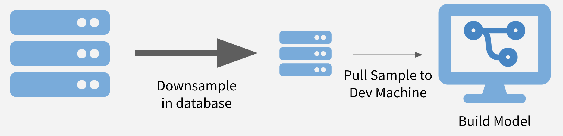
Illustration of Sample and Model
Advantages
- Speed Relative to working on your entire data set, working on just a sample can drastically decrease run times and increase iteration speed.
- Prototyping Even if you’ll eventually have to run your model on the entire data set, this can be a good way to refine hyperparameters and do feature engineering for your model.
- Packages Since you’re working on a normal in-memory data set, you can use all your favorite R packages.
Disadvantages
- Sampling Downsampling isn’t terribly difficult, but does need to be done with care to ensure that the sample is valid and that you’ve pulled enough points from the original data set.
- Scaling If you’re using sample and model to prototype something that will later be run on the full data set, you’ll need to have a strategy (such as pushing compute to the data) for scaling your prototype version back to the full data set.
- Totals Business Intelligence (BI) tasks frequently answer questions about totals, like the count of all sales in a month. One of the other strategies is usually a better fit in this case.
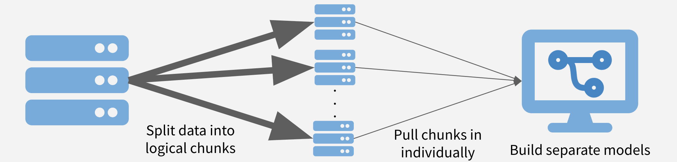
Strategy 2: Chunk and Pull
In this strategy, the data is chunked into separable units and each chunk is pulled separately and operated on serially, in parallel, or after recombining. This strategy is conceptually similar to the MapReduce algorithm. Depending on the task at hand, the chunks might be time periods, geographic units, or logical like separate businesses, departments, products, or customer segments.
Chunk and Pull Illustration
Advantages
- Full data set The entire data set gets used.
- Parallelization If the chunks are run separately, the problem is easy to treat as embarassingly parallel and make use of parallelization to speed runtimes.
Disadvantages
- Need Chunks Your data needs to have separable chunks for chunk and pull to be appropriate.
- Pull All Data Eventually have to pull in all data, which may still be very time and memory intensive.
- Stale Data The data may require periodic refreshes from the database to stay up-to-date since you’re saving a version on your local machine.
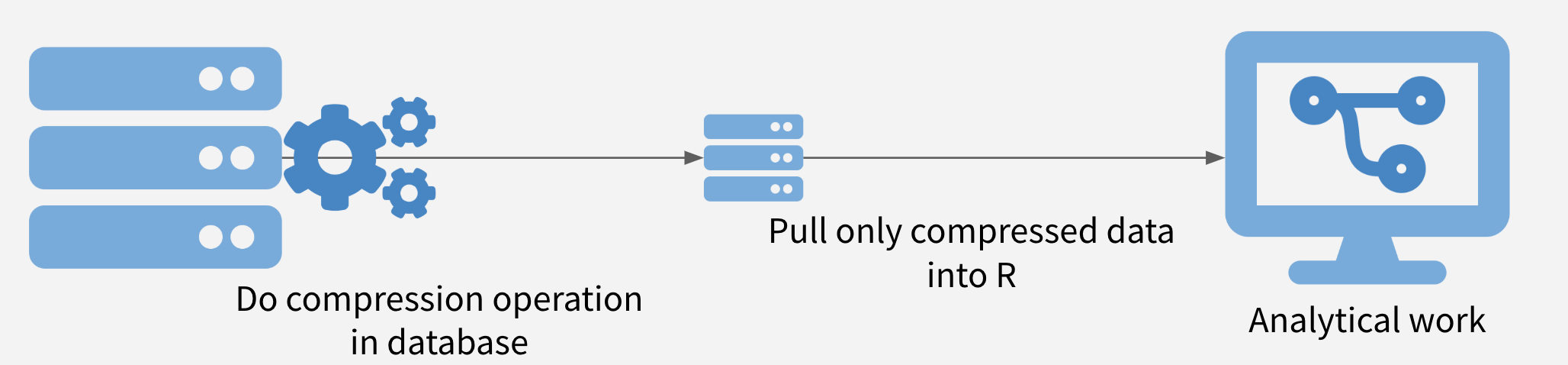
Strategy 3: Push Compute to Data
In this strategy, the data is compressed on the database, and only the compressed data set is moved out of the database into R. It is often possible to obtain significant speedups simply by doing summarization or filtering in the database before pulling the data into R.
Sometimes, more complex operations are also possible, including computing histogram and raster maps with dbplot, building a model with modeldb, and generating predictions from machine learning models with tidypredict.
Push Compute to Data Illustration
Advantages
- Use the Database Takes advantage of what databases are often best at: quickly summarizing and filtering data based on a query.
- More Info, Less Transfer By compressing before pulling data back to R, the entire data set gets used, but transfer times are far less than moving the entire data set.
Disadvantages
- Database Operations Depending on what database you’re using, some operations might not be supported.
- Database Speed In some contexts, the limiting factor for data analysis is the speed of the database itself, and so pushing more work onto the database is the last thing analysts want to do.
An Example
I’ve preloaded the flights data set from the nycflights13 package into a PostgreSQL database, which I’ll use for these examples.
Let’s start by connecting to the database. I’m using a config file here to connect to the database, one of RStudio’s recommended database connection methods:
library(DBI)
library(dplyr)
library(ggplot2)

db <- DBI::dbConnect(
  odbc::odbc(),
  Driver = config$driver,
  Server = config$server,
  Port = config$port,
  Database = config$database,
  UID = config$uid,
  PWD = config$pwd,
  BoolsAsChar = ""
)
The dplyr package is a great tool for interacting with databases, since I can write normal R code that is translated into SQL on the backend. I could also use the DBI package to send queries directly, or a SQL chunk in the R Markdown document.
df <- dplyr::tbl(db, "flights")
tally(df)
## # A tibble: 1 x 1
## n
## <int>
## 1 336776With only a few hundred thousand rows, this example isn’t close to the kind of big data that really requires a Big Data strategy, but it’s rich enough to demonstrate on.
Sample and Model
Let’s say I want to model whether flights will be delayed or not. This is a great problem to sample and model.
Let’s start with some minor cleaning of the data
# Create is_delayed column in database
df <- df %>%
  mutate(
    # Create is_delayed column
    is_delayed = arr_delay > 0,
    # Get just hour (currently formatted so 6 pm = 1800)
    hour = sched_dep_time / 100
  ) %>%
  # Remove small carriers that make modeling difficult
  filter(!is.na(is_delayed) & !carrier %in% c("OO", "HA"))


df %>% count(is_delayed)
## # A tibble: 2 x 2
## is_delayed n
## <lgl> <int>
## 1 FALSE 194078
## 2 TRUE 132897These classes are reasonably well balanced, but since I’m going to be using logistic regression, I’m going to load a perfectly balanced sample of 40,000 data points.
For most databases, random sampling methods don’t work super smoothly with R, so I can’t use dplyr::sample_n or dplyr::sample_frac. I’ll have to be a little more manual.
set.seed(1028)

# Create a modeling dataset
df_mod <- df %>%
  # Within each class
  group_by(is_delayed) %>%
  # Assign random rank (using random and row_number from postgres)
  mutate(x = random() %>% row_number()) %>%
  ungroup()

# Take first 20K for each class for training set
df_train <- df_mod %>%
  filter(x <= 20000) %>%
  collect()

# Take next 5K for test set
df_test <- df_mod %>%
  filter(x > 20000 & x <= 25000) %>%
  collect()

# Double check I sampled right
count(df_train, is_delayed)
count(df_test, is_delayed)
## # A tibble: 2 x 2
## is_delayed n
## <lgl> <int>
## 1 FALSE 20000
## 2 TRUE 20000## # A tibble: 2 x 2
## is_delayed n
## <lgl> <int>
## 1 FALSE 5000
## 2 TRUE 5000Now let’s build a model – let’s see if we can predict whether there will be a delay or not by the combination of the carrier, the month of the flight, and the time of day of the flight.
mod <- glm(is_delayed ~ carrier +
             as.character(month) +
             poly(sched_dep_time, 3),
           family = "binomial",
           data = df_train)

# Out-of-Sample AUROC
df_test$pred <- predict(mod, newdata = df_test)
auc <- suppressMessages(pROC::auc(df_test$is_delayed, df_test$pred))
auc
## Area under the curve: 0.6425As you can see, this is not a great model and any modelers reading this will have many ideas of how to improve what I’ve done. But that wasn’t the point!
I built a model on a small subset of a big data set. Including sampling time, this took my laptop less than 10 seconds to run, making it easy to iterate quickly as I want to improve the model. After I’m happy with this model, I could pull down a larger sample or even the entire data set if it’s feasible, or do something with the model from the sample.
Chunk and Pull
In this case, I want to build another model of on-time arrival, but I want to do it per-carrier. This is exactly the kind of use case that’s ideal for chunk and pull. I’m going to separately pull the data in by carrier and run the model on each carrier’s data.
I’m going to start by just getting the complete list of the carriers.
# Get all unique carriers
carriers <- df %>%
  select(carrier) %>%
  distinct() %>%
  pull(carrier)
Now, I’ll write a function that
- takes the name of a carrier as input
- pulls the data for that carrier into R
- splits the data into training and test
- trains the model
- outputs the out-of-sample AUROC (a common measure of model quality)
carrier_model <- function(carrier_name) {
  # Pull a chunk of data
  df_mod <- df %>%
    dplyr::filter(carrier == carrier_name) %>%
    collect()

  # Split into training and test
  split <- df_mod %>%
    rsample::initial_split(prop = 0.9, strata = "is_delayed") %>%
    suppressMessages()

  # Get training data
  df_train <- split %>% rsample::training()

  # Train model
  mod <- glm(is_delayed ~ as.character(month) + poly(sched_dep_time, 3),
             family = "binomial",
             data = df_train)

  # Get out-of-sample AUROC
  df_test <- split %>% rsample::testing()
  df_test$pred <- predict(mod, newdata = df_test)
  suppressMessages(auc <- pROC::auc(df_test$is_delayed ~ df_test$pred))

  auc
}
Now, I’m going to actually run the carrier model function across each of the carriers. This code runs pretty quickly, and so I don’t think the overhead of parallelization would be worth it. But if I wanted to, I would replace the lapply call below with a parallel backend.3
set.seed(98765)
mods <- lapply(carriers, carrier_model) %>%
  suppressMessages()

names(mods) <- carriers
Let’s look at the results.
mods## $UA
## Area under the curve: 0.6408
##
## $AA
## Area under the curve: 0.6041
##
## $B6
## Area under the curve: 0.6475
##
## $DL
## Area under the curve: 0.6162
##
## $EV
## Area under the curve: 0.6419
##
## $MQ
## Area under the curve: 0.5973
##
## $US
## Area under the curve: 0.6096
##
## $WN
## Area under the curve: 0.6968
##
## $VX
## Area under the curve: 0.6969
##
## $FL
## Area under the curve: 0.6347
##
## $AS
## Area under the curve: 0.6906
##
## $`9E`
## Area under the curve: 0.6071
##
## $F9
## Area under the curve: 0.625
##
## $YV
## Area under the curve: 0.7029So these models (again) are a little better than random chance. The point was that we utilized the chunk and pull strategy to pull the data separately by logical units and building a model on each chunk.
Push Compute to the Data
In this case, I’m doing a pretty simple BI task - plotting the proportion of flights that are late by the hour of departure and the airline.
Just by way of comparison, let’s run this first the naive way – pulling all the data to my system and then doing my data manipulation to plot.
system.time(
  df_plot <- df %>%
    collect() %>%
    # Change is_delayed to numeric
    mutate(is_delayed = ifelse(is_delayed, 1, 0)) %>%
    group_by(carrier, sched_dep_time) %>%
    # Get proportion per carrier-time
    summarize(delay_pct = mean(is_delayed, na.rm = TRUE)) %>%
    ungroup() %>%
    # Change string times into actual times
    mutate(sched_dep_time = stringr::str_pad(sched_dep_time, 4, "left", "0") %>%
             strptime("%H%M") %>%
             as.POSIXct())) -> timing1
Now that wasn’t too bad, just 2.366 seconds on my laptop.
But let’s see how much of a speedup we can get from chunk and pull. The conceptual change here is significant - I’m doing as much work as possible on the Postgres server now instead of locally. But using dplyr means that the code change is minimal. The only difference in the code is that the collect call got moved down by a few lines (to below ungroup()).
system.time(
  df_plot <- df %>%
    # Change is_delayed to numeric
    mutate(is_delayed = ifelse(is_delayed, 1, 0)) %>%
    group_by(carrier, sched_dep_time) %>%
    # Get proportion per carrier-time
    summarize(delay_pct = mean(is_delayed, na.rm = TRUE)) %>%
    ungroup() %>%
    collect() %>%
    # Change string times into actual times
    mutate(sched_dep_time = stringr::str_pad(sched_dep_time, 4, "left", "0") %>%
             strptime("%H%M") %>%
             as.POSIXct())) -> timing2
It might have taken you the same time to read this code as the last chunk, but this took only 0.269 seconds to run, almost an order of magnitude faster!4 That’s pretty good for just moving one line of code.
Now that we’ve done a speed comparison, we can create the nice plot we all came for.
df_plot %>%
  mutate(carrier = paste0("Carrier: ", carrier)) %>%
  ggplot(aes(x = sched_dep_time, y = delay_pct)) +
  geom_line() +
  facet_wrap("carrier") +
  ylab("Proportion of Flights Delayed") +
  xlab("Time of Day") +
  scale_y_continuous(labels = scales::percent) +
  scale_x_datetime(date_breaks = "4 hours",
                   date_labels = "%H")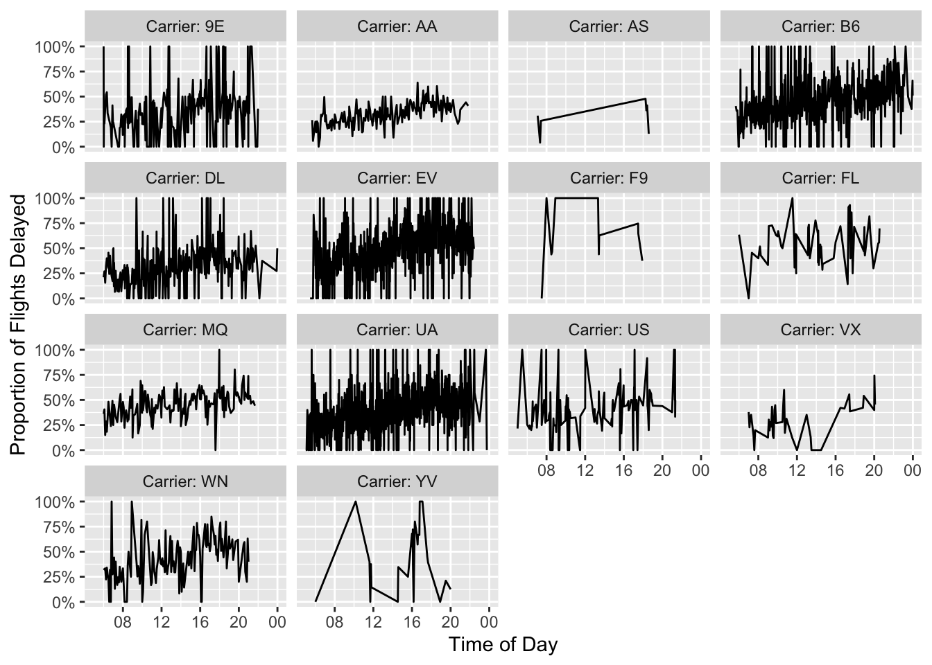
It looks to me like flights later in the day might be a little more likely to experience delays, but that’s a question for another blog post.
https://blog.codinghorror.com/the-infinite-space-between-words/↩
This isn’t just a general heuristic. You’ll probably remember that the error in many statistical processes is determined by a factor of \(\frac{1}{n^2}\) for sample size \(n\), so a lot of the statistical power in your model is driven by adding the first few thousand observations compared to the final millions.↩
One of the biggest problems when parallelizing is dealing with random number generation, which you use here to make sure that your test/training splits are reproducible. It’s not an insurmountable problem, but requires some careful thought.↩
And lest you think the real difference here is offloading computation to a more powerful database, this Postgres instance is running on a container on my laptop, so it’s got exactly the same horsepower behind it.↩
You may leave a comment below or discuss the post in the forum community.rstudio.com.