This is a guest post from Gary Hutson, lead of Machine Learning at Crisp Thinking, a company that provides AI solutions to moderate and detect offensive and abusive content online. His website is available at https://hutsons-hacks.info/ and he can be reached through Twitter, @StatsGary.
MLDataR package motivation
I love all things Machine Learning. The MLDataR package was driven by the need to have example datasets across the healthcare system for machine learning problems. I have been a machine learning practitioner for over nine years; however, I still find it interesting to explore new examples and datasets related to supervised machine learning classification and regression.
Because the package contains clinical examples and examples from real hospital systems, it allows the potential machine learning engineer to practice all things related to supervised machine learning.
Despite the package initially being aimed at healthcare, I have expanded it to new territories and domains.
What does the package contain?
The package contains several datasets for modelling. This is just a start and I am working with the NHS-R community to build it out even further. It is a sort of a call to arms to equip the package with even more examples of excellent datasets that can be used for machine learning.
Diabetes disease prediction - This dataset contains key variables, gathered from hospital research and papers in the British Medical Journal to identify the drivers behind diabetes disease. This dataset is useful for working with supervised classification machine learning problems or statistical problems. It uses past historical patient information to train and classify a model, with the aim to classify if a patient will have diabetes when they first present to the service.
Diabetes early onset - Gathered by Asif Laldin, the package contributor from Gloucestershire Clinical Commissioning Group, this dataset contains information on the time between a prediabetes diagnosis and the onset of diabetes.
Failing care home prediction - Using measures from the NHS incident reporting databases, this dataset contains data to classify if a care home will fail based on results from retrospective inspections.
Heart disease prediction - This dataset is intended for supervised machine learning classification problems on which patients are likely to present with heart disease. This uses independent variables, such as resting blood pressure, maximum heart rate, history of angina, and other metrics.
Thyroid disease classification - This one has a personal effect on me, as I am a sufferer of this disease. This drove me to source this dataset from the Garavan Institute, based on a collection of studies this institute did around thyroid disease. This contains 28 independent or predictor variables of patients with or without the disease. It is also covered in the vignette supporting this package and the supporting YouTube tutorial using tidymodels with various ML techniques.
Counter Strike Global Offensive (CSGO) - This dataset was kindly contributed by Asif Laldin, and is a detraction from the healthcare datasets in the package. I never intended the package to be purely healthcare ML datasets, and I plan to include credit card fraud examples, tabular playground examples from Kaggle, and many more, so watch this space…
Run a tidymodels routine with heart disease dataset
Let’s explore the heart disease dataset contained in MLDataR using a logistic regression model.
# install.packages("MLDataR")
library(MLDataR)
library(dplyr)
library(tidyr)
library(tidymodels)
library(data.table)
library(ConfusionTableR)
library(OddsPlotty)
glimpse(MLDataR::heartdisease)
## Rows: 918
## Columns: 10
## $ Age <dbl> 40, 49, 37, 48, 54, 39, 45, 54, 37, 48, 37, 58, 39, 4…
## $ Sex <chr> "M", "F", "M", "F", "M", "M", "F", "M", "M", "F", "F"…
## $ RestingBP <dbl> 140, 160, 130, 138, 150, 120, 130, 110, 140, 120, 130…
## $ Cholesterol <dbl> 289, 180, 283, 214, 195, 339, 237, 208, 207, 284, 211…
## $ FastingBS <dbl> 0, 0, 0, 0, 0, 0, 0, 0, 0, 0, 0, 0, 0, 0, 0, 0, 0, 0,…
## $ RestingECG <chr> "Normal", "Normal", "ST", "Normal", "Normal", "Normal…
## $ MaxHR <dbl> 172, 156, 98, 108, 122, 170, 170, 142, 130, 120, 142,…
## $ Angina <chr> "N", "N", "N", "Y", "N", "N", "N", "N", "Y", "N", "N"…
## $ HeartPeakReading <dbl> 0.0, 1.0, 0.0, 1.5, 0.0, 0.0, 0.0, 0.0, 1.5, 0.0, 0.0…
## $ HeartDisease <dbl> 0, 1, 0, 1, 0, 0, 0, 0, 1, 0, 0, 1, 0, 1, 0, 0, 1, 0,…A glimpse into the dataset gives us a quick overview of our dataset. We have 918 rows and 10 columns. We can see our outcome, heart disease, and our nine predictors.
There are a couple of things we want to clean up. Notice that our outcome variable HeartDisease loads as a double variable. We want to convert it into a factor variable for our machine learning model.
The variables Sex, RestingECG, and AnginaY are character variables. For creating models, it is better to encode characters as factors.
hd <- heartdisease %>%
  mutate(across(where(is.character), as.factor),
         HeartDisease = as.factor(HeartDisease)) %>%
  # Remove any non complete cases
  na.omit()
is.factor(hd$HeartDisease)
## [1] TRUEFor Machine Learning models, it is generally recommended to split your data into a training and testing set, or if you are using hyperparameter tuning and updating your model, a training / test and validation set. Other methods are available, such a K-Fold Cross Validation; however, we will stick to a basic training and testing split for the purposes of this walkthrough.
To do this, and to make sure that the results are repeatable, we will use the set.seed(123) value - which essentially says when we are randomly splitting this data, make sure that the random pattern is the same as the walkthrough., i.e. give me the same split as this post:
set.seed(123)
split_prop <- 0.8
testing_prop <- 1 - split_prop
split <- rsample::initial_split(hd, prop = split_prop)
training <- rsample::training(split)
testing <- rsample::testing(split)
# Print a custom message to show the samples involved
training_message <- function() {
  message(
    cat(
      'The training set has: ',
      nrow(training),
      ' examples and the testing set has:',
      nrow(testing),
      '.\nThis split has ',
      paste0(format(100 * split_prop), '%'),
      ' in the training set and ',
      paste0(format(100 * testing_prop), '%'),
      ' in the testing set.',
      sep = ''
    )
  )
}
training_message()
## The training set has: 734 examples and the testing set has:184.
## This split has 80% in the training set and 20% in the testing set.## We can fit a parsnip model to the training set and then we can evaluate the performance.
lr_hd_fit <- logistic_reg() %>%
  set_engine("glm") %>%
  set_mode("classification") %>%
  fit(HeartDisease ~ ., data = training)
If we want to see the summary results of our model in a tidy way (i.e., a data frame with standard column names), we can use the tidy() function:
tidy(lr_hd_fit)## # A tibble: 11 × 5
## term estimate std.error statistic p.value
## <chr> <dbl> <dbl> <dbl> <dbl>
## 1 (Intercept) 0.925 1.29 0.718 4.73e- 1
## 2 Age 0.0175 0.0123 1.42 1.55e- 1
## 3 SexM 1.17 0.241 4.84 1.29e- 6
## 4 RestingBP -0.00164 0.00544 -0.301 7.63e- 1
## 5 Cholesterol -0.00335 0.00104 -3.23 1.25e- 3
## 6 FastingBS 0.944 0.248 3.81 1.39e- 4
## 7 RestingECGNormal -0.291 0.261 -1.12 2.64e- 1
## 8 RestingECGST -0.383 0.343 -1.12 2.64e- 1
## 9 MaxHR -0.0192 0.00450 -4.28 1.88e- 5
## 10 AnginaY 1.54 0.229 6.72 1.78e-11
## 11 HeartPeakReading 0.689 0.113 6.12 9.54e-10We can see the statistically significant ones by pulling out those with p < 0.05: Male (SexM), cholesterol (Cholesterol), fasting blood sugar (FastingBS), maximum heart rate (MaxHR), having angina (AnginaY), and peak heart rate reading (HeartPeakReading).
tidy(lr_hd_fit) %>%
  filter(p.value < 0.05) %>%
  pull(term)
## [1] "SexM" "Cholesterol" "FastingBS" "MaxHR"
## [5] "AnginaY" "HeartPeakReading"Let’s convert the probabilities from the fitted GLM model into odds ratios (ORs). An OR measures the association between an exposure and an outcome.1 In this case, the OR represents the odds of heart disease will occur given a particular condition, compared to the odds of heart disease occurring in the absence of that condition.
We can visualize the results using the OddsPlotty package and the fit list object from the model.
tidy_oddsplot <- OddsPlotty::odds_plot(
  lr_hd_fit$fit,
  title = "Heart Disease Odds Plot",
  point_col = "#6b95ff",
  h_line_color = "red"
)
tidy_oddsplot <- tidy_oddsplot$odds_plot +
  theme(legend.position = "none") +
  geom_text(
    label = round(tidy_oddsplot$odds_plot$data$OR, digits = 3),
    hjust = -0.5,
    vjust = 1,
    cex = 2.8
  )
tidy_oddsplot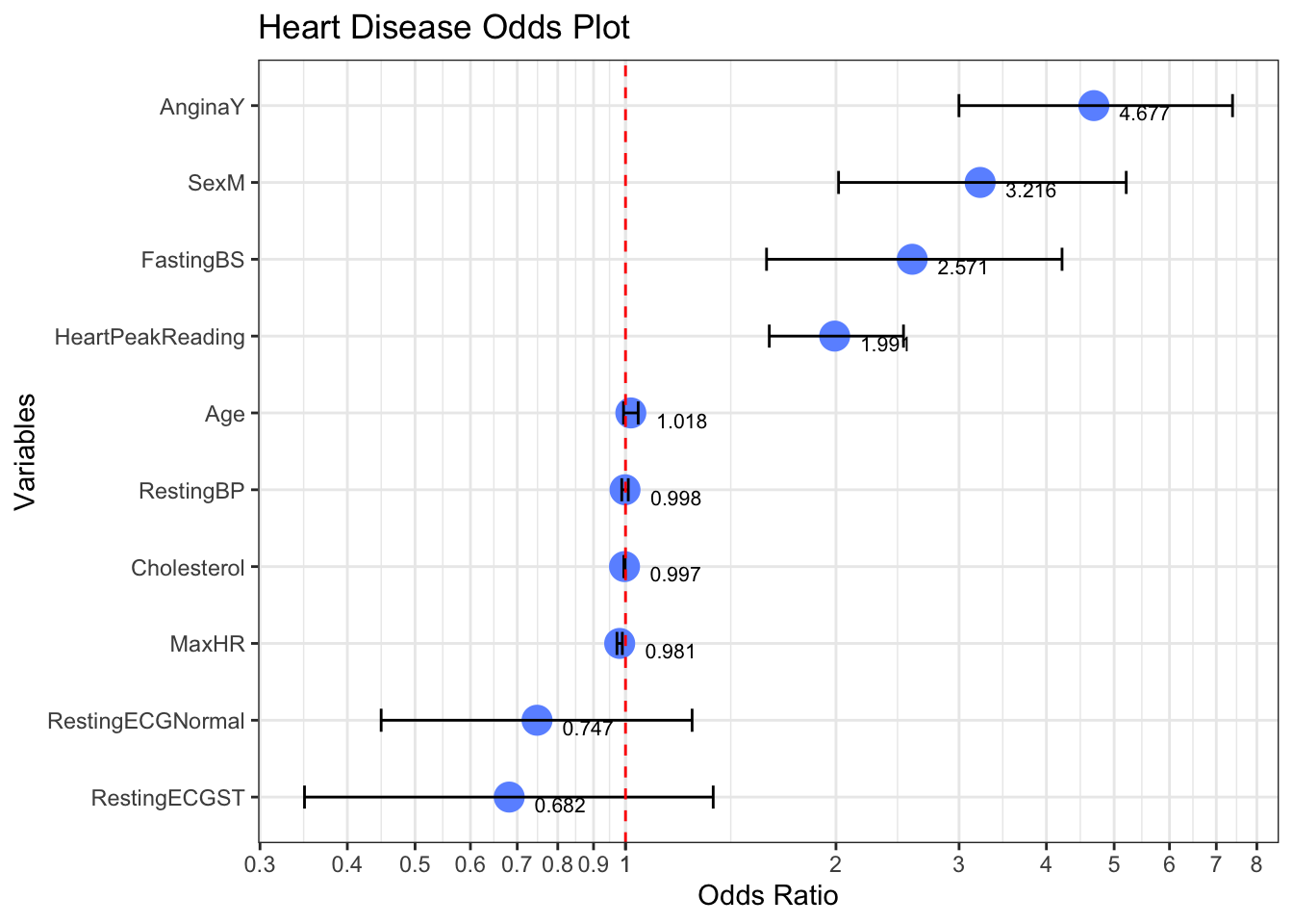
We can also pull out the odds ratio data:
tidy_oddsplot$data## OR lower upper vars
## Age 1.0176 0.9935 1.0426 Age
## SexM 3.2156 2.0172 5.2026 SexM
## RestingBP 0.9984 0.9877 1.0090 RestingBP
## Cholesterol 0.9967 0.9946 0.9987 Cholesterol
## FastingBS 2.5710 1.5912 4.2114 FastingBS
## RestingECGNormal 0.7472 0.4471 1.2452 RestingECGNormal
## RestingECGST 0.6817 0.3474 1.3348 RestingECGST
## MaxHR 0.9809 0.9722 0.9895 MaxHR
## AnginaY 4.6768 2.9989 7.3842 AnginaY
## HeartPeakReading 1.9914 1.6056 2.4982 HeartPeakReadingIn this example, odds ratios are used to compare the relative odds of the occurrence of heart disease, given exposure to the variable of interest. Looking at the results from odds_plot():
Having angina (AnginaY), peak heart rate reading (HeartPeakReading), Male (SexM), and fasting blood sugar (FastingBS) have an OR of greater than 1, implying that these conditions are associated with higher odds of heart disease. For example, people with Angina are 4.677 times more likely to get heart disease than those without this condition.
Normal resting electrocardiogram (RestingECGNormal) and normal ST segment of an electrocardiogram (RestingECGST) have an OR of less than 1, implying that these conditions are associated with lower odds of heart disease, however due to the length of the error bars these conditions do not have as significant effect on heart disease, as those outlined with odds greater than 1.
Note the confidence intervals, indicating the precision of the OR. The large CIs around RestingECGNormal and RestingECGST indicate a low level of precision of the OR. The small CIs around Age, RestingBP, Cholesterol, and MaxHRindicate a higher precision of the ORs. This is normally due to the representation of the encoded items within the model, i.e. the presence of an effect code.
I evaluate the outputs of logistic regression models by using the sampling probability values that the variables have been selected by chance (p-values) for the cut off, but then use the odds ratios of the effect of the predictor variable on my outcome, using the odds plots to make the final decision.
Evaluating with testing set
The final way we can evaluate how well our model fits, before pushing this into production, would be to use a confusion matrix to collect how well our testing partition performs, against our training model predictions. Here we are trying to get a sense of, if we pushed this into the wild, how well would it do on unseen observations i.e. those new items that we don’t have a label for, a label in this sense is whether someone has had heart disease, or not.
library(ConfusionTableR)
# Use our model to predict labels on to testing set
predictions <- cbind(predict(lr_hd_fit, new_data = testing),
                     testing)
# Create confusion matrix and output to record level for storage to monitor concept drift
cm <- ConfusionTableR::binary_class_cm(
  predictions$.pred_class,
  predictions$HeartDisease,
  mode = 'everything',
  positive = '1'
)
## [INFO] Building a record level confusion matrix to store in dataset## [INFO] Build finished and to expose record level cm use the record_level_cm list itemThe next step is to expose the confusion matrix to view how well our model did on estimating the labels on the testing set:
# Access the confusion matrix list object
cm$confusion_matrix
## Confusion Matrix and Statistics
##
## Reference
## Prediction 0 1
## 0 70 6
## 1 16 92
##
## Accuracy : 0.88
## 95% CI : (0.825, 0.924)
## No Information Rate : 0.533
## P-Value [Acc > NIR] : <2e-16
##
## Kappa : 0.758
##
## Mcnemar's Test P-Value : 0.055
##
## Sensitivity : 0.939
## Specificity : 0.814
## Pos Pred Value : 0.852
## Neg Pred Value : 0.921
## Precision : 0.852
## Recall : 0.939
## F1 : 0.893
## Prevalence : 0.533
## Detection Rate : 0.500
## Detection Prevalence : 0.587
## Balanced Accuracy : 0.876
##
## 'Positive' Class : 1
## Our model did relatively well. Picking apart some of the metrics:
- True positives (
TP) we have 92 correctly classified instances of heart failure - True negatives(
TN) we have 70 cases classified as not having heart disease - False negatives (
FN) we have 6 cases were our model said the patient didn’t have heart disease and they did - False positives (
FP) we have 16 cases were our model said a patient did have heart disease, but they actually didn’t - Recall (also called Sensitivity) is 0.9388 meaning from all the patients that had heart disease - how many did we predict correctly - this equation is
Recall=TP / (TP + FN) - Precision (also called Positive Predictive Value) is 0.8519 meaning from all the classes we predicted as positive, how many were actually positive. The equation here is
Precision=TP/(TP + FP).
As I run many ML experiments, I wanted a way to store this data into a record-level extract. I actually stored this in a model metrics table on Postgres SQL database, but could be stored in any proprietary system. To get these metrics easily in record level, the package I created helps you do that with ease:
# As we used the binary record level cm method, this stores the model data down
record_level_cm <- cm$record_level_cm %>%
  dplyr::mutate(user_name = Sys.getenv("USERNAME"))
glimpse(record_level_cm)
## Rows: 1
## Columns: 24
## $ Pred_0_Ref_0 <int> 70
## $ Pred_1_Ref_0 <int> 16
## $ Pred_0_Ref_1 <int> 6
## $ Pred_1_Ref_1 <int> 92
## $ Accuracy <dbl> 0.8804
## $ Kappa <dbl> 0.7581
## $ AccuracyLower <dbl> 0.8246
## $ AccuracyUpper <dbl> 0.9235
## $ AccuracyNull <dbl> 0.5326
## $ AccuracyPValue <dbl> 4.902e-24
## $ McnemarPValue <dbl> 0.05501
## $ Sensitivity <dbl> 0.9388
## $ Specificity <dbl> 0.814
## $ Pos.Pred.Value <dbl> 0.8519
## $ Neg.Pred.Value <dbl> 0.9211
## $ Precision <dbl> 0.8519
## $ Recall <dbl> 0.9388
## $ F1 <dbl> 0.8932
## $ Prevalence <dbl> 0.5326
## $ Detection.Rate <dbl> 0.5
## $ Detection.Prevalence <dbl> 0.587
## $ Balanced.Accuracy <dbl> 0.8764
## $ cm_ts <dttm> 2022-04-19 11:18:51
## $ user_name <chr> ""#Export to csv
data.table::fwrite(record_level_cm, file = 'heart_disease_cm_record_level.csv')If you were happy with your model now, you could put this into production.
Can I contribute my own dataset to MLDataR?
The answer is you can, and I would greatly encourage it. To boot, you will become a package contributor. I am looking for ML datasets from across a wide range of industries and organisations.
Suitable datasets for machine learning applications:
- Have sufficient predictive variables for feature engineering
- Have a nominal outcome variable
- May have missing values
- Consist of interesting features
If you have an idea, please submit a pull request to the GitHub repository and add your dataset.
Final thoughts
I have really enjoyed putting this package together and I hope you can use it to:
Learn tidymodels or caret. I have put together a few tutorials on these in the past:
- Building a tidymodels classification model from scratch: https://www.youtube.com/watch?v=hxRx7ozLNKw&t=2583s
- Advanced modelling with caret for supervised machine learning: https://www.youtube.com/watch?v=rO40vvKXU-4&t=3085s
- Reticulate - R and Python a happy union: https://www.youtube.com/watch?v=8WE-EU5k97Q&t=235s
- Collapsing a caret confusion matrix with ConfusionTableR: https://youtu.be/9zcUlgLySZo
Put your models into production:
- Deploying a caret machine learning model as an API with Plumber: https://youtu.be/WMCkV_J5a0s
- Creating a microservice with Docker and serving as a restful API: https://youtu.be/JK6VLAKRjO4
Szumilas M. (2010). Explaining odds ratios. Journal of the Canadian Academy of Child and Adolescent Psychiatry = Journal de l’Academie canadienne de psychiatrie de l’enfant et de l’adolescent, 19(3), 227–229.↩︎
You may leave a comment below or discuss the post in the forum community.rstudio.com.