Today, we change gears from our previous work on Fama French and run a Monte Carlo (MC) simulation of future portfolio returns. Monte Carlo relies on repeated, random sampling. We will sample based on two parameters: mean and standard deviation of portfolio returns. Our long-term goal (long-term == over the next two or three blog posts) is to build a Shiny app that allows an end user to build a custom portfolio, simulate returns and visualize the results. If you just can’t wait, a link to that final Shiny app is here.
Let’s get to it.
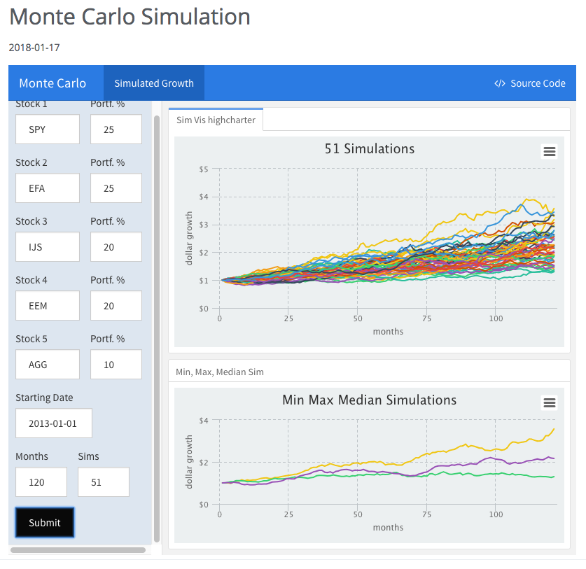
Devoted readers won’t be surprised that we will be simulating the returns of our usual portfolio, which consists of:
+ SPY (S&P 500 fund) weighted 25%
+ EFA (a non-US equities fund) weighted 25%
+ IJS (a small-cap value fund) weighted 20%
+ EEM (an emerging-mkts fund) weighted 20%
+ AGG (a bond fund) weighted 10%
Before we can simulate that portfolio, we need to calculate portfolio monthly returns, which was covered in my previous post, Introduction to Portfolio Returns.
I won’t go through the logic again, but the code is here:
library(tidyquant)
library(tidyverse)
library(timetk)
library(broom)

symbols <- c("SPY","EFA", "IJS", "EEM","AGG")

prices <-
  getSymbols(symbols, src = 'yahoo',
             from = "2012-12-31",
             to = "2017-12-31",
             auto.assign = TRUE, warnings = FALSE) %>%
  map(~Ad(get(.))) %>%
  reduce(merge) %>%
  `colnames<-`(symbols)

w <- c(0.25, 0.25, 0.20, 0.20, 0.10)

asset_returns_long <-
  prices %>%
  to.monthly(indexAt = "lastof", OHLC = FALSE) %>%
  tk_tbl(preserve_index = TRUE, rename_index = "date") %>%
  gather(asset, returns, -date) %>%
  group_by(asset) %>%
  mutate(returns = (log(returns) - log(lag(returns)))) %>%
  na.omit()

portfolio_returns_tq_rebalanced_monthly <-
  asset_returns_long %>%
  tq_portfolio(assets_col  = asset,
               returns_col = returns,
               weights     = w,
               col_rename  = "returns",
               rebalance_on = "months")
We will be working with the data object portfolio_returns_tq_rebalanced_monthly and we first find the mean and standard deviation of returns.
We will name those variables mean_port_return and stddev_port_return.
mean_port_return <-
  mean(portfolio_returns_tq_rebalanced_monthly$returns)

stddev_port_return <-
  sd(portfolio_returns_tq_rebalanced_monthly$returns)
Then we use the rnorm() function to sample from a distribution with mean equal to mean_port_return and standard deviation equal to stddev_port_return. That is the crucial random sampling that underpins this exercise.
We also must decide how many draws to pull from this distribution, meaning how many monthly returns we will simulate. 120 months is 10 years, and that feels like a good amount of time.
simulated_monthly_returns <- rnorm(120,
                                   mean_port_return,
                                   stddev_port_return)
Have a quick look at the simulated monthly returns.
head(simulated_monthly_returns)[1] 0.05216143 0.02271485 -0.04271307 0.04811250 -0.05575058 0.06006096tail(simulated_monthly_returns)[1] 0.024794729 0.008539198 -0.018852629 -0.002656127 -0.025583337
[6] 0.004412755Next, we calculate how a dollar would have grown given those random monthly returns. We first add a 1 to each of our monthly returns, because we start with $1.
simulated_returns_add_1 <-
  tibble(c(1, 1 + simulated_monthly_returns)) %>%
  `colnames<-`("returns")

head(simulated_returns_add_1)
# A tibble: 6 x 1
returns
<dbl>
1 1
2 1.05
3 1.02
4 0.957
5 1.05
6 0.944That data is now ready to be converted into the cumulative growth of a dollar. We can use either accumulate() from purrr or cumprod(). Let’s use both of them with mutate() and confirm consistent, reasonable results.
simulated_growth <-
simulated_returns_add_1 %>%
    mutate(growth1 = accumulate(returns, function(x, y) x * y),
           growth2 = accumulate(returns, `*`),
           growth3 = cumprod(returns)) %>%
    select(-returns)

tail(simulated_growth)
# A tibble: 6 x 3
growth1 growth2 growth3
<dbl> <dbl> <dbl>
1 2.09 2.09 2.09
2 2.11 2.11 2.11
3 2.07 2.07 2.07
4 2.06 2.06 2.06
5 2.01 2.01 2.01
6 2.02 2.02 2.02We just ran three simulations of dollar growth over 120 months. We passed in the same monthly returns, and that’s why we got three equivalent results.
Are they reasonable? What compound annual growth rate (CAGR) is implied by this simulation?
cagr <-
  ((simulated_growth$growth1[nrow(simulated_growth)]^
      (1/10)) - 1) * 100

cagr <- round(cagr, 2)
This simulation implies an annual compounded growth of 7.26%. That seems reasonable given our actual returns have all been taken from a raging bull market. Remember, the above code is a simulation based on sampling from a normal distribution. If you re-run this code on your own, you will get a different result.
If we feel good about this first simulation, we can run several more to get a sense for how they are distributed. Before we do that, let’s create several different functions that could run the same simulation.
Several Simulation Functions
Let’s build three simulation functions that incorporate the accumulate() and cumprod() workflows above. We have confirmed they give consistent results so it’s a matter of stylistic preference as to which one is chosen in the end. Perhaps you feel that one is more flexible or extensible, or fits better with your team’s code flows.
Each of the below functions needs four arguments: N for the number of months to simulate (we chose 120 above), init_value for the starting value (we used $1 above), and the mean-standard deviation pair to create draws from a normal distribution. We choose N and init_value, and derive the mean-standard deviation pair from our portfolio monthly returns.
Here is our first growth simulation function using accumulate().
simulation_accum_1 <- function(init_value, N, mean, stdev) {
    tibble(c(init_value, 1 + rnorm(N, mean, stdev))) %>%
    `colnames<-`("returns") %>%
    mutate(growth =
             accumulate(returns,
                        function(x, y) x * y)) %>%
    select(growth)
}
Almost identical, here is the second simulation function using accumulate().
simulation_accum_2 <- function(init_value, N, mean, stdev) {
  tibble(c(init_value, 1 + rnorm(N, mean, stdev))) %>%
    `colnames<-`("returns") %>%
  mutate(growth = accumulate(returns, `*`)) %>%
  select(growth)
}
Finally, here is a simulation function using cumprod().
simulation_cumprod <- function(init_value, N, mean, stdev) {
  tibble(c(init_value, 1 + rnorm(N, mean, stdev))) %>%
    `colnames<-`("returns") %>%
  mutate(growth = cumprod(returns)) %>%
  select(growth)
}
Here is a function that uses all three methods, in case we want a fast way to re-confirm consistency.
simulation_confirm_all <- function(init_value, N, mean, stdev) {
  tibble(c(init_value, 1 + rnorm(N, mean, stdev))) %>%
    `colnames<-`("returns") %>%
    mutate(growth1 = accumulate(returns, function(x, y) x * y),
           growth2 = accumulate(returns, `*`),
           growth3 = cumprod(returns)) %>%
    select(-returns)
}
Let’s test that confirm_all() function with an init_value of 1, N of 120, and our parameters.
simulation_confirm_all_test <-
  simulation_confirm_all(1, 120,
                         mean_port_return, stddev_port_return)

tail(simulation_confirm_all_test)
# A tibble: 6 x 3
growth1 growth2 growth3
<dbl> <dbl> <dbl>
1 2.26 2.26 2.26
2 2.22 2.22 2.22
3 2.17 2.17 2.17
4 2.21 2.21 2.21
5 2.20 2.20 2.20
6 2.23 2.23 2.23That’s all for today. Next time, we will explore methods for running more than one simulation with the above functions and then visualizing the results. See you then.
You may leave a comment below or discuss the post in the forum community.rstudio.com.